Motivation
Over the past twenty years, political campaign expenditures in the United States have skyrocketed. In 1998, these expenditures amounted to $1.6 billion. In 2018, this number is projected to hit $5.2 billion (Center for Responsive Politics). This effect is often credited to the controversial 2010 Citizens United decision, which effectively prohibited the United States government from restricting independent expenditures for political communications. However, this upward trend in expenditures began long before 2010. Importantly, we can infer from this pattern that political professionals see a direct causal relationship between campaign expenditures and electoral outcomes.
Many prior studies of campaign spending are limited in scope, and often concern elections in the 1970s and 1980s. Additionally, the preponderance of existing scholarship focuses mainly on the effects of incumbency. In this study, I examine the shape and the form of the relationship between campaign expenditures and campaign efficacy with several sets of controls in place. I use a comprehensive set of data encompassing all House of Representatives elections between 2006 and 2016.
I look to develop a comprehensive picture of campaign spending in the 21st century through two main avenues. First, I analyze the overall relationship between spending and voting as denominated in dollars and votes. Second, I examine competitive dynamics within districts through the analysis of candidate spending share, which is defined as the candidate’s spending divided by all spending by candidates in the district. In this branch of my analysis, I compare spending share to vote share.
Literature Review
The first body of scholarship consulted was the literature surrounding the relationship between campaign spending and electoral outcomes. This work has mainly focused on the effects of incumbency. In 1978, Gary Jacobson established that the marginal utility of campaign spending is different for incumbents than it is for challengers. Challengers often begin their campaigns in relative obscurity and can quickly boost their public profiles through high levels of campaign spending. Incumbents, on the other hand, can leverage their established political networks and extensive communication resources to develop name recognition and support outside of the formal campaign spending process. In 1985, Jacobson argues that “no matter how the data are analyzed, no matter what view one takes of the simultaneity problem, one finding remains undisturbed: incumbents gain nothing in the way of votes by spending money in campaigns.”
This conclusion has been debated extensively. In their 1988 paper, Green and Krasno argue that Jacobson failed to control for challenger quality, pertinent interaction effects, and reciprocal causation. Green and Krasno incorporate prior incumbent spending as an exogenous variable to identify the incumbent’s general propensity to spend. Green and Krasno arrive at the conclusion that incumbents can readily affect their vote share by spending on the margin. In 1990, Jacobson responded, claiming that Green and Krasno’s model incorporates a high degree of multicollinearity, as their prior incumbent spending instrument correlates highly with the challenger political quality and expenditure variables in the model. Jacobson argues that the instrument for incumbent spending “is, in part, a proxy for party strength and challenger quality.” One goal of my study is to re-examine this debate in the context of the modern campaign finance landscape.
I also rely on scholarship surrounding election forecasting. In 2014, Patrick Hummel and David Rothschild explored the usage of econometric modeling to forecast campaign outcomes. Specifically, they focus on presidential, gubernatorial, and senatorial races. Hummel and Rothschild use presidential approval ratings, incumbency, past election results, economic factors, and state ideology to predict electoral outcomes. They find that past election results, incumbency, and state-level economic factors can be used to predict electoral outcomes with a high degree of statistical significance. Consequently, I use both past election results and incumbency in my models. I exclude economic factors for two reasons. First, I was unable to acquire district-level personal income data in the timeframe of this project. Second, I follow the example of FiveThirtyEight’s 2018 House forecast, which did not include economic factors. Indirectly, voters’ economic attitudes and opinions are incorporated into the model through generic ballot polling. In my model, cycle-level fixed effects also likely pick up some of this noise.
Based on FiveThirtyEight’s usage of generic ballot polling, I decided to include a generic ballot measure in my models. I use a variation of the technique described by Joseph Bafumi, Robert S. Erikson, and Christopher Wlezien in their 2008 paper, in which they average all generic ballot polls over the last 30 days of a given campaign, converting all polls to a percent Democratic of the two-party vote. For instance, 50-42 converts to 54.3% Democratic. I interact this variable with a factor variable for political party to capture the obvious differences in the ways that Democrat-favorable polling affects candidates of different parties.
Data, Hypotheses, and Methods
Data
I use publicly available Federal Election Commission and generic ballot data for this study. The FEC data was downloaded directly from the FEC’s official website. The generic ballot data was downloaded from the Analyzing Polling and Election Data in R course on DataCamp and was initially compiled by G. Elliott Morris of The Economist. The initial candidate and disbursement dataset consisted of all candidates for the United States House of Representatives in elections between 2004 and 2016. Some exclusions were made. All candidates without vote counts or disbursement numbers were removed. Additionally, all candidates for office in United States territories were excluded, as these officials cannot vote on the House floor. There were also several duplicate records for individual candidates within the initial dataset. These were condensed or removed as necessary.
In his 1991 study of incumbency and campaign spending, Alan Abramowitz included a variable for district partisanship. In this case, the variable described how the district voted in the previous presidential election. District-level presidential election data for the timeframe of my study exists but is not freely available. In future extensions of this study, I will attempt to procure this data. In the meantime, I chose to include a Previous Democratic Share variable, which shows the Democratic candidate’s share of the district vote in the previous election. The inclusion of this variable necessitated dropping all 2004 data from these analyses.
In all, 5049 observations were included in the final analyses. Two detailed breakdowns of this data can be found below.
In the first table, the data are broken out by cycle and summarized into relevant spending and electoral outcome statistics. We see that the average and median candidate’s votes are highest in presidential election years, which makes intuitive sense given the well-documented trend of higher voter turnout in presidential years. On the disbursement side, we see that both median and average disbursements remained relatively consistent between 2006 and 2016. This consistency is present even in presidential years. Finally, we see that candidates of the opposition party tend to poll well, as Democrats held a generic ballot advantage in 2006 and 2008, and Republicans held an advantage in all Obama-era elections outside of 2012.
The second table shows the data broken down by both party and cycle
In the second table, the data are further broken out by party, to show spending and outcome differences within cycles and between parties. There are some slight discrepancies from officially published election results here, mainly due to the analytically problematic observations deleted during the data cleaning. I continue to work through the data set to identify all potential inaccuracies. We see in this table that Republicans tend to outspend Democrats. For Democrats and Republicans, we also see that average vote and disbursement numbers tend to be higher than their respective medians, indicating a rightward skew.
Hypotheses
Based on the literature reviewed, I test three hypotheses. The first two are outlined below, and serve to analyze Jacobson, Green, and Krasno’s work in the context of the modern campaign finance landscape.
H1: With respect to campaign expenditures, both win probability and votes won will increase at a decreasing rate. That is, I predict a diminishing marginal utility of campaign expenditures.
H2: The shape and form of this relationship, and consequently the point of zero marginal utility will change depending on the affiliation of the candidate, partisan makeup of the district, the national political climate, and challenger or incumbent status of the candidate.
The third hypothesis relies on a different conception of the relationship between spending and votes. Specifically, I look to analyze the relationship between spending share and vote share. To my knowledge, this specific analysis has not been performed. Spending share is defined here as a candidate’s spending divided by the total spending of all candidates in that specific race.
H3: Share of spending will correlate positively with vote share, but the shape of this relationship will be different than in H1. This is because opponent spending and vote share is more effectively controlled for within this design.
Methods
I test all three of these hypotheses with linear regression. My linear regressions incorporate fixed effects at the cycle and district level. This means that different intercept terms are generated based on each election’s location and year. Theoretically, these fixed effects should control for time-invariant differences between districts and location-invariant differences between years. In future extensions of this inquiry I plan on generating random effects, interacting specific independent variables with district and cycle to further control for differences between districts and years.
I run three regressions analyzing the relationship between dollars spent and votes won, and I also run three regressions analyzing the relationship between share of spending and share of votes won. The third and final regression of each of these series is the most complete and is primarily used in my analyses.
The equations for the two critical regressions are shown below. TotDisbM refers to candidate disbursements denominated in millions of dollars. ShareofSpend refers to a candidate’s share of spending. The incumbent variable is a dummy variable, with incumbents assigned the value of 1. MeanDemShareGenBallot is the mean Democratic share of all generic ballot polls conducted within 30 days of the election. Party is a five-level factor variable, with 0 representing Democrats, 1 representing Republicans, 2 representing Libertarians, 3 representing Green Party members, and 4 representing all other and independent candidates. OthDistDisbM refers to the sum of spending by other candidates competing in the race in question. PartyInPres is a dummy variable, with the value 1 being assigned to candidates in the same party as the sitting president. DemSharePrior refers to the vote share won by the Democratic candidate in the prior House election in the district in question.
Dollars Spent-Votes Won Regression
\(Votes Won = \beta_0 + \beta_{1} TotDisb + \beta_{2}Incumbent + \beta_{3}MeanDemShareGenBall + \beta_{4}Republican + \beta_{5}Libertarian + \beta_{6}Green + \beta_{7}Other\) \(+ \beta_{8}OthDistDisbM +\beta_{9}PartyinPres + \beta_{10}DemSharePrior + \beta_{11}TotDisbM*Incumbent + \beta_{12}MeanDemShareGenBall*Republican\) \(+ \beta_{13}MeanDemShareGenBall*Libertarian + \beta_{14}MeanDemShareGenBall*Green + \beta_{15}MeanDemShareGenBall*Other\) \(+ \beta_{16}DemSharePrior*Republican + \beta_{17}DemSharePrior*Libertarian + \beta_{18}DemSharePrior*Green + \beta_{19}DemSharePrior*Other\)
Results
Dollars and Votes
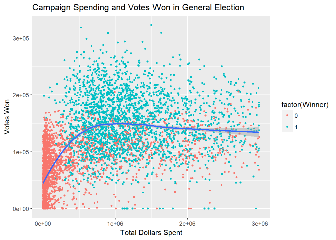
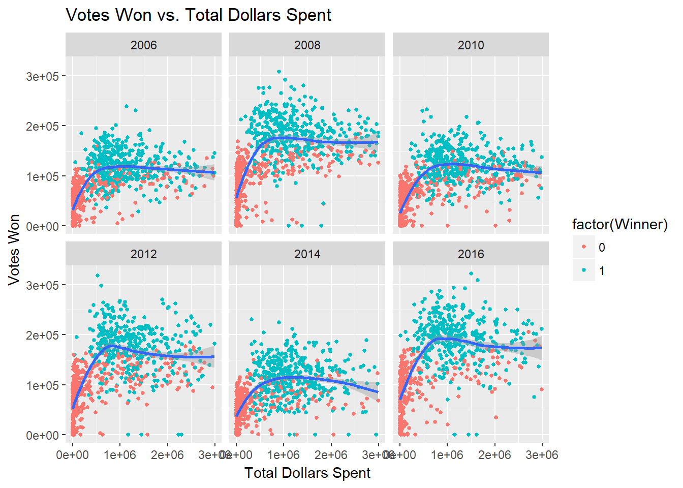
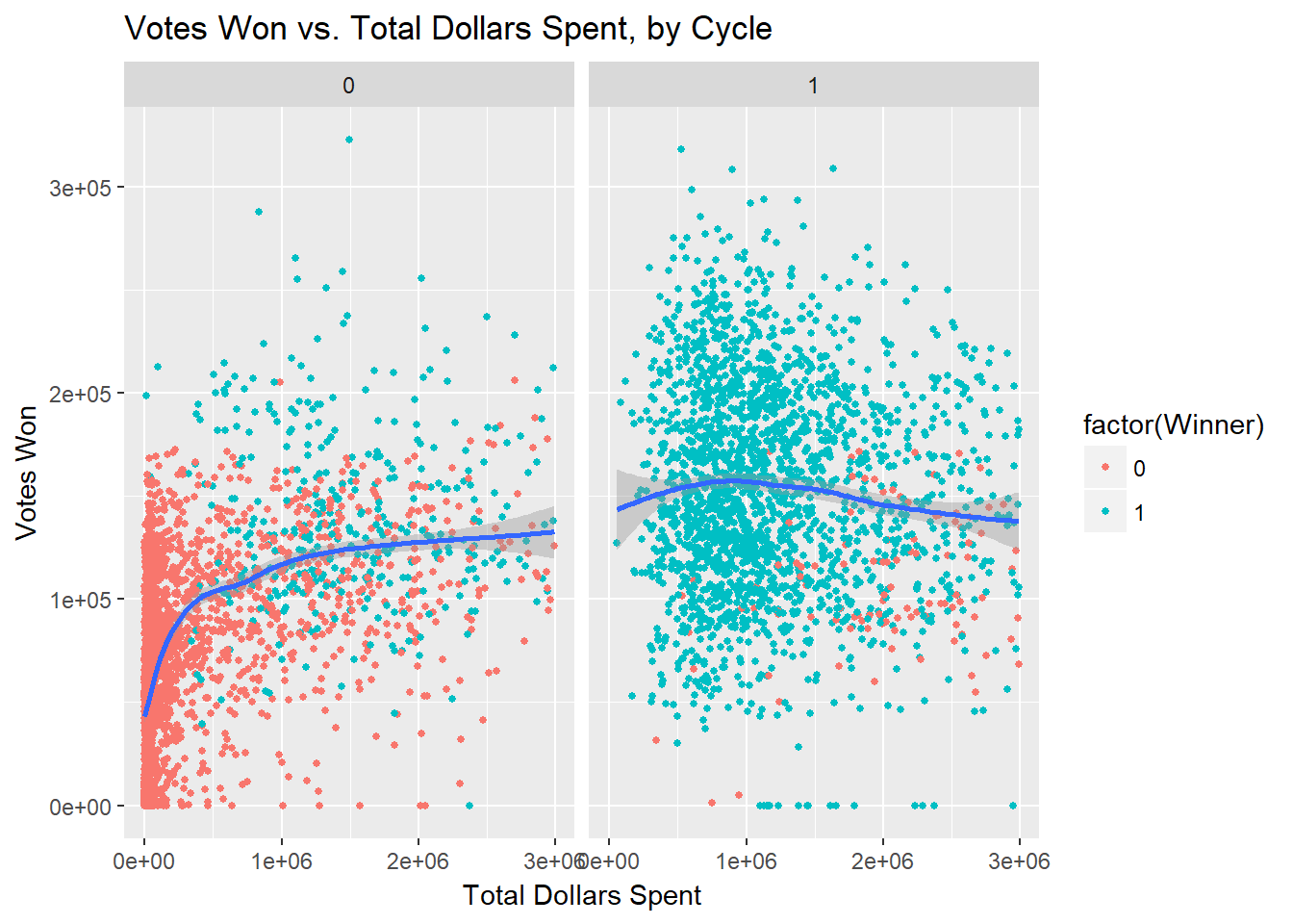
In the following three charts, a reduced dataset is used. This dataset eliminates spending outliers to show a clearer picture of the relationships depicted. The fitted lines should not be affected, as they are fitted by locally estimated scatterplot smoothing models.
In the first figure, we see the relationship between dollars spent and votes won. Clearly, this chart represents a severely declining marginal utility of campaign spending with respect to votes won. Although there are no controls in place here, the basic inference could be made that campaign spending past the $1 million mark may be irrational.

Below, I break out this relationship by cycle. Two trends jump out here. First, we see that the fitted line moves upward in presidential years. This makes intuitive sense. Presidential elections generally boast higher turnout than midterm elections. With a higher expected vote count, each dollar spent in presidential years corresponds to more votes won than each dollar spent in midterm elections. The second key takeaway here is that the plateau point is roughly the same in all years. In other words, the marginal utility of campaign spending approaches zero at roughly the same spending point in all six elections.

Finally, I separate non-incumbent candidates from incumbent candidates below. These data confirm Jacobson’s 1978 conclusion that the relationship between campaign spending and votes won behaves differently for incumbents than it does for non-incumbents. More specifically, two conclusions can be made here. First, incumbents are far more likely to win than non-incumbents. Second, we see that higher spending by incumbents actually corresponds with a lower number of votes won. This may be due to higher spending by incumbents in more competitive elections. This supports Jacobson’s findings.

Next, I run three regressions with votes won as the dependent variable and dollars spent as the independent variable of interest. The third regression is the most comprehensive and is used for this analysis. All dependent variables other than mean Democratic share of generic ballot, Libertarian party status, and Green party status interacted with Democratic share in prior election are highly statistically significant.
Critically, we see that the total disbursement incumbent interaction is both negative and greater in magnitude than the (positive) total disbursement estimate. This means that with all controls in place, our model predicts that challengers face a generally positive marginal utility of spending while incumbents face a generally negative marginal utility of spending. This further supports Jacobson’s findings concerning incumbency and spending.
| Dependent variable: | |||
| Votes Won | |||
| (1) | (2) | (3) | |
| TotDisbM | 17,016.370*** | 18,273.100*** | 16,079.390*** |
| (617.315) | (619.950) | (617.320) | |
| factor(Incumbent)1 | 74,310.530*** | 70,538.730*** | 58,761.240*** |
| (1,221.378) | (1,251.112) | (1,423.221) | |
| MeanDemShareGenBall | 385,816.500 | 375,430.100 | 375,208.200 |
| (350,810.600) | (351,384.600) | (348,734.100) | |
| factor(Party)1 | 140,659.800*** | 136,338.000*** | 164,232.400*** |
| (13,085.690) | (12,946.310) | (14,893.740) | |
| factor(Party)2 | 58,974.810 | 44,333.980 | 42,993.390 |
| (52,140.260) | (51,572.760) | (53,451.680) | |
| factor(Party)3 | 183,347.300*** | 199,106.500*** | 207,426.800*** |
| (65,451.170) | (64,734.190) | (63,167.810) | |
| factor(Party)4 | 93,746.650*** | 109,880.600*** | 103,858.900*** |
| (25,250.570) | (25,007.130) | (25,159.650) | |
| OthDistDisbM | -3,341.656*** | -3,075.836*** | |
| (291.251) | (284.352) | ||
| factor(PartyInPres)1 | -2,288.637* | ||
| (1,281.758) | |||
| DemSharePrior | 25,629.230*** | ||
| (3,200.957) | |||
| TotDisbM:factor(Incumbent)1 | -19,468.030*** | -20,110.060*** | -17,397.210*** |
| (762.838) | (756.323) | (753.761) | |
| MeanDemShareGenBall:factor(Party)1 | -276,677.400*** | -268,738.200*** | -263,504.400*** |
| (25,862.220) | (25,585.280) | (28,295.080) | |
| MeanDemShareGenBall:factor(Party)2 | -260,037.600** | -225,954.100** | -213,614.400** |
| (105,493.400) | (104,355.600) | (104,788.300) | |
| MeanDemShareGenBall:factor(Party)3 | -493,405.900*** | -518,799.100*** | -540,511.400*** |
| (126,353.900) | (124,961.600) | (124,013.800) | |
| MeanDemShareGenBall:factor(Party)4 | -319,266.000*** | -345,244.800*** | -330,475.100*** |
| (50,217.830) | (49,706.840) | (48,887.690) | |
| factor(Party)1:DemSharePrior | -70,503.010*** | ||
| (4,336.888) | |||
| factor(Party)2:DemSharePrior | -25,766.410* | ||
| (13,208.590) | |||
| factor(Party)3:DemSharePrior | -11,566.560 | ||
| (16,744.910) | |||
| factor(Party)4:DemSharePrior | -18,199.660*** | ||
| (6,706.886) | |||
| Constant | -113,101.400 | -102,705.700 | -107,754.000 |
| (177,709.100) | (178,001.300) | (176,688.600) | |
| Observations | 5,049 | 5,049 | 5,049 |
| Log Likelihood | -59,417.410 | -59,345.970 | -59,152.960 |
| Akaike Inf. Crit. | 118,866.800 | 118,725.900 | 118,351.900 |
| Bayesian Inf. Crit. | 118,971.200 | 118,836.900 | 118,502.000 |
| Note: | p<0.1; p<0.05; p<0.01 | ||
Discussion
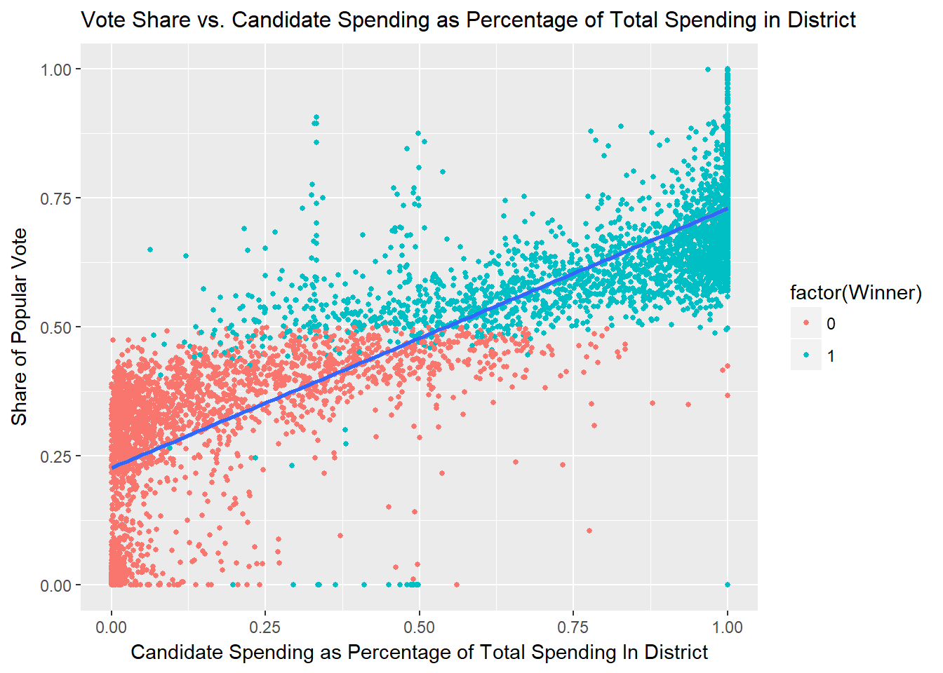
I report two main findings. First, on a high level, I find a severely diminishing marginal relationship between campaign spending and votes won, with the curve flattening out just before the $1 million mark. For incumbents, the marginal utility of spending is negative. Second, I observe a strong, positive, and highly linear relationship between candidates’ share of spending within their district and their respective share of the vote. This effect is highly significant. I control for incumbency, generic ballot polling, party affiliation, opponent spending, and district partisanship, and I generate fixed effects for district and cycle.
Framed in terms of my initial hypotheses, we see that all three hypotheses are supported by the data. The first hypothesis posits that candidates will face a diminishing marginal utility of campaign spending. When denominated in dollars spent and votes won, the marginal utility of campaign spending indeed appears to decline rapidly, approaching the zero point at around $1 million. The second hypothesis is also supported by the data. In my regressions, party affiliation, Democratic share in the prior election, and incumbent status are all statistically significant. Democratic share of generic ballot is only significant when interacted with party. Importantly, we observe that incumbents face a negative marginal utility of campaign spending. Finally, the third hypothesis asserts that the share of spending will correlate with vote share, but that the relationship will look different than in the first hypothesis. This is also supported. We observe a highly linear relationship between a candidate’s share of spending and their ultimate share of the vote.
There is an important conflict between the results of the dollars spent-votes won analysis and the results of the spending share-vote share analysis. The dollars spent-votes won regression shows a positive marginal utility of spending for non-incumbents and a negative marginal utility of spending for incumbents. This supports Jacobson’s view. However, the spending share-vote share regression shows a non-significant interaction between incumbent status and share of spending. This supports Green and Krasno’s finding that, with the proper effects in place, incumbents can significantly affect their chances of winning by spending more.
The dollars spent-votes won examines candidates on an individual basis, with opponent spending included as a covariate. In contrast, the spending share variable captures a candidate’s spending in terms of total activity by candidates in the district, just as the vote share variable captures a candidate’s results in terms of all results in the race. When results are expressed as vote share, a vote for Candidate A is mathematically largely offset by a vote for their opponent. Importantly, vote share is what ultimately matters for election results. When spending is expressed as spending share, a dollar spent by Candidate A is mathematically largely offset by a dollar spent by Candidate A’s opponent. As such, I argue that the spending share-vote share comparison better captures the competitive dynamics at play. Consequently, I find a strong and linear relationship between spending share and vote share.
The findings yielded by the two analyses can help explain political professionals’ heavy focus on campaign fundraising and spending. The dollars spent-votes won comparison indicates that there is nearly zero marginal utility past roughly the first $1 million spent. This would indicate that the existing high levels of fundraising and spending are irrational. However, the spending share-vote share comparison suggests that a given candidate’s marginal dollar spent is always spent rationally, so long that the candidate is increasing their share of district spending. By observing campaign spending through the lens of spending share and vote share, we can empirically examine and evaluate modern trends in campaign spending. While dollars spent may offer a diminishing marginal utility, candidates can always stand to benefit by outspending their opponent to the greatest extent possible.
Limitations and Next Steps
I plan on continuing to analyze this data, pursuing both extensions of the present research inquiry and entirely new projects. One clear limitation in my present analysis is my lack of attention to the simultaneity problem. As Gary Jacobson explains in his 1990 paper, campaign donations are often made in response to electoral expectations. At the same time, campaign spending often translates to a higher probability of victory for challengers and a lower probability of victory for incumbents. This is because endangered incumbents often engage in more vigorous fundraising, and promising challengers are provided with funds by hopeful supporters. This simultaneous causation leads to some estimation problems, as it is difficult to parse out the direction of causality. In their 1994 paper, Goidel and Gross attempt to deal with this issue through a three-stage least squares design, modeling incumbent and challenger expenditures as endogenous variables through a simultaneous system of equations. My design does not directly address the simultaneity problem. As such, my estimates may be prone to systematic bias driven by simultaneous causality. However, in future extensions of this design, I look to incorporate an adapted version of Goidel and Gross’ three-stage least squares design.
Another extension that I may pursue is the incorporation of logistic regression into my analyses. In these regressions, the dependent variable would be the logged odds of victory. By directly analyzing the impact of campaign spending on probability of victory, I may be able to generate more intuitive and useful results than simply looking at votes and vote share.
Finally, I look to dig more into the potential impact of Citizens United on campaign spending. While I’ve explored this in a roundabout way through my disaggregation of the dollars spent-votes won trend into the different cycles, I do not focus specifically on the impact of this decision. While I considered including a supplemental analysis of the impact of Citizens United into this project, I ultimately decided that such an important topic would be ill-suited as an analytical afterthought. Consequently, I will look to explore this in a future project.
References
Abramowitz, A.I. 1991. “Campaign Spending, and the Decline of Competition in U.S. House Elections.” The Journal of Politics 53 (1).
Bafumi, J., R.S. Erikson, and C. Wlezien. 2008. “Forecasting House Seats from Generic Congressional Polls.” Elections and Exit Polling.
Gerber, A.S. 2004. “Does Campaign Spending Work? Field Experiments Provide Evidence and Suggest New Theory.” American Behavioral Scientist 47 (5).
Goidel, R.K., and D.A. Gross. 1994. “A Systems Approach to Campaign Finance in U.S. House.” American Politics Quarterly 22 (2).
Green, D.P., and J.S. Krasno. 1988. “Salvation for the Spendthrift Incumbent: Reestimating the Effects of Campaign Spending in House Elections.” American Journal of Political Science 32 (4).
Hlavac, Marek. 2018. Stargazer: Well-Formatted Regression and Summary Statistics Tables. Bratislava, Slovakia: Central European Labour Studies Institute (CELSI). https://CRAN.R-project.org/package=stargazer.
Hummel, P., and D. Rothschild. 2014. “Fundamental Models for Forecasting Elections at the State Level.” Electoral Studies.
Jacobson, G.C. 1990. “The Effects of Campaign Spending in House Elections: New Evidence for Old Arguments.” American Journal of Political Science 34 (2).
Morris, G.E. n.d. “Analyzing Election and Polling Data in R.” https://www.datacamp.com/courses/analyzing-election-and-polling-data-in-r; DataCamp.
Silver, N. 2018. “How Fivethirtyeight’s House Model Works.” https://fivethirtyeight.com/features/2018-house-forecast-methodology/; FiveThirtyEight.
2018. https://www.opensecrets.org/news/2018/10/2018-midterm-record-breaking-5-2-billion/; Center for Responsive Politics.
